GRAFOS - GRAPH K-MEANS

GRAFOS = (V, E) siendo V = Vértices, E = Edges, Aristas.

TIPOS DE GRAFOS

GRAFO TRIVIAL	GRAFO SIMPLE
GRAFO PONDERADO	GRAFO DIRIGIDO
GRAFO MULTIGRAFO	GRAFO COMPLETO

GRAFO DIRIGIDO

CLUSTERING TASK

HIERARCHICAL CLUSTERING METHODS

k-MEANS CLUSTERING

EXAMPLE OF k-MEANS CLUSTERING AT WORK

APPLICATION OF k-MEANS CLUSTERING USING SAS ENTERPRISE MINER

USING CLUSTER MEMBERSHIP TO PREDICT CHURN


CLUSTERING TASK

Clustering refers to the grouping of records, observations, or cases into classes of similar objects. A cluster is a collection of records that are similar to one another and dissimilar to records in other clusters. Clustering differs from classification in that there is no target variable for clustering. The clustering task does not try to classify, estimate, or predict the value of a target variable. Instead, clustering algorithms seek to segment the entire data set into relatively homogeneous subgroups or clusters, where the similarity of the records within the cluster is maximized, and the similarity to records outside this cluster is minimized.

For example, Claritas, Inc. is a clustering business that provides demographic

profiles of each geographic area in the United States, as defined by zip code. One of the clustering mechanisms they use is the PRIZM segmentation system, which describes every U.S. zip code area in terms of distinct lifestyle types. Recall, for example, that the clusters identified for zip code 90210, Beverly Hills, California, were:

• Cluster 01: Blue Blood Estates
• Cluster 10: Bohemian Mix
• Cluster 02: Winner’s Circle
• Cluster 07: Money and Brains
• Cluster 08: Young Literati

The description for cluster 01: Blue Blood Estates is “Established executives,

professionals, and ‘old money’ heirs that live in America’s wealthiest suburbs. They are accustomed to privilege and live luxuriously—one-tenth of this group’s members are multimillionaires. The next affluence level is a sharp drop from this pinnacle.”

Examples of clustering tasks in business and research include:

• Target marketing of a niche product for a small-capitalization business that does not have a large marketing budget.
• For accounting auditing purposes, to segment financial behavior into benign and suspicious categories.
• As a dimension-reduction tool when a data set has hundreds of attributes.
• For gene expression clustering, where very large quantities of genes may exhibit similar behavior.

Clustering is often performed as a preliminary step in a data mining process,

with the resulting clusters being used as further inputs into a different technique

downstream, such as neural networks. Due to the enormous size of many present-day databases, it is often helpful to apply clustering analysis first, to reduce the search space for the downstream algorithms. In this chapter, after a brief look at hierarchical clustering methods, we discuss in detail k-means clustering; in Chapter 9 we examine clustering using Kohonen networks, a structure related to neural networks.

Cluster analysis encounters many of the same issues that we dealt with in the

chapters on classification. For example, we shall need to determine:

• How to measure similarity
• How to recode categorical variables
• How to standardize or normalize numerical variables
• How many clusters we expect to uncover

 For simplicity, in this book we concentrate on Euclidean distance between

records:

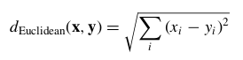
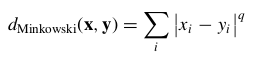
 where x = x 1 , x 2 , . . . , x m , and y = y 1 , y 2 , . . . , y m represent the m attribute values of two records. Of course, many other metrics exist, such as city-block distance:

or Minkowski distance, which represents the general case of the foregoing two metrics for a general exponent q:



 For categorical variables, we may again define the “different from” function for

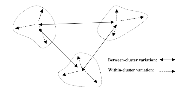
 Figure 8.1 Clusters should have small within-cluster variation compared to the between-cluster variation.

Comparing the ith attribute values of a pair of records:

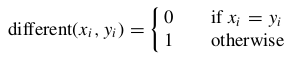
where x i and y i are categorical values. We may then substitute different(x i , y i) for the ith term in the Euclidean distance metric above.

For optimal performance, clustering algorithms, just like algorithms for classi-

fication, require the data to be normalized so that no particular variable or subset of variables dominates the analysis. Analysts may use either the min–max normalization or Z-score standardization, discussed in earlier chapters:

All clustering methods have as their goal the identification of groups of records

such that similarity within a group is very high while the similarity to records in other groups is very low. In other words, as shown in Figure 8.1, clustering algorithms seek to construct clusters of records such that the between-cluster variation (BCV) is large compared to the within-cluster variation (WCV) This is somewhat analogous to the concept behind analysis of variance.

HIERARCHICAL CLUSTERING METHODS

Clustering algorithms are either hierarchical or nonhierarchical. In hierarchical clustering, a treelike cluster structure (dendrogram) is created through recursive partitioning (divisive methods) or combining (agglomerative) of existing clusters. Agglomerative clustering methods initialize each observation to be a tiny cluster of its own.

Then, in succeeding steps, the two closest clusters are aggregated into a new

combined cluster. In this way, the number of clusters in the data set is reduced by one at each step. Eventually, all records are combined into a single huge cluster. Divisive clustering methods begin with all the records in one big cluster, with the most dissimilar records being split off recursively, into a separate cluster, until each record represents its own cluster. Because most computer programs that apply hierarchical clustering use agglomerative methods, we focus on those.

Distance between records is rather straightforward once appropriate recoding

and normalization has taken place. But how do we determine distance between clusters of records? Should we consider two clusters to be close if their nearest neighbors are close or if their farthest neighbors are close? How about criteria that average out these extremes?

We examine several criteria for determining distance between arbitrary clusters

A and B:

• Single linkage, sometimes termed the nearest-neighbor approach, is based on the minimum distance between any record in cluster A and any record in cluster B. In other words, cluster similarity is based on the similarity of the most similar members from each cluster. Single linkage tends to form long, slender clusters, which may sometimes lead to heterogeneous records being clustered together.
• Complete linkage, sometimes termed the farthest-neighbor approach, is  based on the maximum distance between any record in cluster A and any record in cluster B. In other words, cluster similarity is based on the similarity of the most dissimilar members from each cluster. Complete-linkage tends to form more compact, spherelike clusters, with all records in a cluster within a given diameter of all other records. 
• Average linkage is designed to reduce the dependence of the cluster-linkage
  criterion on extreme values, such as the most similar or dissimilar records.
  In average linkage, the criterion is the average distance of all the records in
  cluster A from all the records in cluster B. The resulting clusters tend to have approximately equal within-cluster variability. 

Let’s examine how these linkage methods work, using the following small,

one-dimensional data set:

2  5  9  15  16  18  25  33  33  45

Single-Linkage Clustering

Suppose that we are interested in using single-linkage agglomerative clustering on this data set. Agglomerative methods start by assigning each record to its own cluster. Then, single linkage seeks the minimum distance between any records in two clusters. Figure 8.2 illustrates how this is accomplished for this data set. The minimum cluster distance is clearly between the single-record clusters which each contain the value 33, for which the distance must be zero for any valid metric. Thus, these two clusters are combined into a new cluster of two records, both of value 33, as shown in Figure 8.2.

Note that, after step 1, only nine (n − 1) clusters remain. Next, in step 2, the clusters.

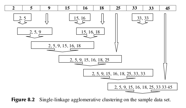
containing values 15 and 16 are combined into a new cluster, since their distance of 1 is the minimum between any two clusters remaining.

Here are the remaining steps:

• Step 3: The cluster containing values 15 and 16 (cluster {15,16}) is combined with cluster {18}, since the distance between 16 and 18 (the closest records in each cluster) is two, the minimum among remaining clusters.
• Step 4: Clusters {2} and {5} are combined.
• Step 5: Cluster {2,5} is combined with cluster {9}, since the distance between 5 and 9 (the closest records in each cluster) is four, the minimum among remaining clusters. 
• Step 6: Cluster {2,5,9} is combined with cluster {15,16,18}, since the distance between 9 and 15 is six, the minimum among remaining clusters. 
• Step 7: Cluster {2,5,9,15,16,18} is combined with cluster {25}, since the distance between 18 and 25 is seven, the minimum among remaining clusters.
• Step 8: Cluster {2,5,9,15,16,18,25} is combined with cluster {33,33}, since the distance between 25 and 33 is eight, the minimum among remaining clusters.
• Step 9: Cluster {2,5,9,15,16,18,25,33,33} is combined with cluster {45}. This last cluster now contains all the records in the data set.

 Complete-Linkage Clustering

Next, let’s examine whether using the complete-linkage criterion would result in a different clustering of this sample data set. Complete linkage seeks to minimize the distance among the records in two clusters that are farthest from each other. Figure 8.3 illustrates complete-linkage clustering for this data set.

• Step 1: Since each cluster contains a single record only, there is no difference between single linkage and complete linkage at step 1. The two clusters each containing 33 are again combined.

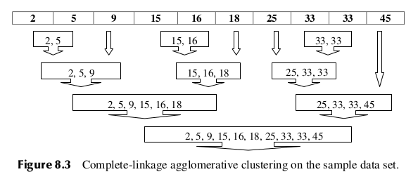
• Step 2: Just as for single linkage, the clusters containing values 15 and 16  are combined into a new cluster. Again, this is because there is no difference in the two criteria for single-record clusters.
• Step 3: At this point, complete linkage begins to diverge from its predecessor. In single linkage, cluster {15,16} was at this point combined with cluster {18}. But complete linkage looks at the farthest neighbors, not the nearest neighbors. The farthest neighbors for these two clusters are 15 and 18, for a distance of 3. This is the same distance separating clusters {2} and {5}. The complete-linkage criterion is silent regarding ties, so we arbitrarily select the first such combination found, therefore combining the clusters {2} and {5} into a new cluster.
• Step 4: Now cluster {15,16} is combined with cluster {18}.
• Step 5: Cluster {2,5} is combined with cluster {9}, since the complete-linkage distance is 7, the smallest among remaining clusters. 
• Step 6: Cluster {25} is combined with cluster {33,33}, with a complete-linkage distance of 8.
• Step 7: Cluster {2,5,9} is combined with cluster {15,16,18}, with a complete-linkage distance of 16.
• Step 8: Cluster {25,33,33} is combined with cluster {45}, with a complete-
  linkage distance of 20. 
• Step 9: Cluster {2,5,9,15,16,18} is combined with cluster {25,33,33,45}. All
  records are now contained in this last large cluster.

Finally, with average linkage, the criterion is the average distance of all the

records in cluster A from all the records in cluster B. Since the average of a single record is the record’s value itself, this method does not differ from the earlier methods in the early stages, where single-record clusters are being combined. At step 3, average linkage would be faced with the choice of combining clusters {2} and {5}, or combining the {15, 16} cluster with the single-record {18} cluster. The average distance between the {15, 16} cluster and the {18} cluster is the average of |18 − 15| and |18 − 16|, which is 2.5, while the average distance between clusters {2} and {5} is of course 3. Therefore, average linkage would combine the {15, 16} cluster with cluster {18} at this step, followed by combining cluster {2} with cluster {5}. The reader may verify that the average-linkage criterion leads to the same hierarchical structure for this example as the complete-linkage criterion. In general, average linkage leads to clusters more similar in shape to complete linkage than does single linkage.

k-MEANS CLUSTERING

The k-means clustering algorithm [1] is a straightforward and effective algorithm for finding clusters in data. The algorithm proceeds as follows.

• Step 1: Ask the user how many clusters k the data set should be partitioned into.
• Step 2: Randomly assign k records to be the initial cluster center locations.
• Step 3: For each record, find the nearest cluster center. Thus, in a sense, each cluster center “owns” a subset of the records, thereby representing a partition of the data set. We therefore have k clusters, C 1 , C 2 , . . . , C k .
• Step 4: For each of the k clusters, find the cluster centroid, and update the location of each cluster center to the new value of the centroid.
• Step 5: Repeat steps 3 to 5 until convergence or termination.

The “nearest” criterion in step 3 is usually Euclidean distance, although other

criteria may be applied as well. The cluster centroid in step 4 is found as fol-

lows. Suppose that we have n data points (A1 , B1 , C1 ), (A2 , B2 , C2 ), . . . , (An, Bn, Cn ), the centroid these points center of gravity of these points and is located at of is the point . For example, the points (1,1,1), (1,2,1), (1,3,1), and (2,1,1) would have centroid.

The algorithm terminates when the centroids no longer change. In other words,

the algorithm terminates when for all clusters C 1 , C 2 , . . . , C k , all the records “owned” by each cluster center remain in that cluster. Alternatively, the algorithm may terminate when some convergence criterion is met, such as no significant shrinkage in the sum of squared errors:

where p ∈ C i represents each data point in cluster i and m i represents the centroid of cluster i.

EXAMPLE OF k-MEANS CLUSTERING AT WORK

Let’s examine an example of how the k-means algorithm works. Suppose that we

have the eight data points in two-dimensional space shown in Table 8.1 and plotted in Figure 8.4 and are interested in uncovering k = 2 clusters.

Let’s apply the k-means algorithm step by step.

• Step 1: Ask the user how many clusters k the data set should be partitioned into. We have already indicated that we are interested in k = 2 clusters.
• Step 2: Randomly assign k records to be the initial cluster center locations. For this example, we assign the cluster centers to be m 1 = (1,1) and m 2 = (2,1). 
• Step 3 (first pass): For each record, find the nearest cluster center. Table 8.2 contains the (rounded) Euclidean distances between each point and each cluster center m 1 = (1,1) and m 2 = (2,1), along with an indication of which cluster center the point is nearest to. Therefore, cluster 1 contains points {a,e,g}, and cluster 2 contains points {b,c,d,f,h}. Once cluster membership is assigned, the sum of squared errors may be found:

As remarked earlier, we would like our clustering methodology to maximize

the between-cluster variation with respect to the within-cluster variation. Using

d(m 1 ,m 2 ) as a surrogate for BCV and SSE as a surrogate for WCV, we have:

We expect this ratio to increase with successive passes.

• Step 4 (first pass): For each of the k clusters find the cluster centroid and update the location of each cluster center to the new value of the centroid. The 

centroid for cluster 1 is [(1 + 1 + 1) /3, (3 + 2 + 1) /3] = (1,2). The centroid

for cluster 2 is [(3 + 4 + 5 + 4 + 2) /5, (3 + 3 + 3 + 2 + 1) /5] = (3.6, 2.4).

The clusters and centroids (triangles) at the end of the first pass are shown in

Figure 8.5. Note that m 1 has moved up to the center of the three points in cluster 1, while m 2 has moved up and to the right a considerable distance, to the center of the five points in cluster 2.

• Step 5: Repeat steps 3 and 4 until convergence or termination. The centroids have moved, so we go back to step 3 for our second pass through the algorithm.
• Step 3 (second pass): For each record, find the nearest cluster center. Table 8.3 shows the distances between each point and each updated cluster center m 1 = (1,2) and m 2 = (3.6, 2.4), together with the resulting cluster membership. There has been a shift of a single record (h) from cluster 2 to cluster 1. The relatively large change in m 2 has left record h now closer to m 1 than to m 2 , so that record h now belongs to cluster 1. All other records remain in the same clusters as previously. Therefore, cluster 1 is {a,e,g,h}, and cluster 2 is {b,c,d,f}. The new sum of squared errors is

which is much reduced from the previous SSE of 36, indicating a better clus-
tering solution. We also have:

 

which is larger than the previous 0.0278, indicating that we are increasing the between-cluster variation with respect to the within-cluster variation.

• Step 4 (second pass): For each of the k clusters, find the cluster centroid and update the location of each cluster center to the new value of the centroid. The new centroid for cluster 1 is [(1 + 1 + 1 + 2)/4, (3 + 2 + 1 +1)/4] = (1.25, 1.75). The new centroid for cluster 2 is [(3 + 4 + 5 + 4)/4, (3 + 3 + 3 + 2)/4] = (4, 2.75). The clusters and centroids at the end of the second pass are shown in Figure 8.6. Centroids m 1 and m 2 have both moved slightly.
• Step 5: Repeat steps 3 and 4 until convergence or termination. Since the centroids have moved, we once again return to step 3 for our third (and as it turns out, final) pass through the algorithm.
• Step 3 (third pass): For each record, find the nearest cluster center. Table 8.4 shows the distances between each point and each newly updated cluster center m 1 = (1.25, 1.75) and m 2 = (4, 2.75), together with the resulting cluster membership. Note that no records have shifted cluster membership from the

which is larger than the previous 0.3338, indicating that we have again increased the between-cluster variation with respect to the within-cluster variation. To do so is the goal of every clustering algorithm, in order to produce well-defined clusters such that the similarity within the cluster is high while the similarity to records in other clusters is low.

• Step 4 (third pass): For each of the k clusters, find the cluster centroid and
  update the location of each cluster center to the new value of the centroid. Since no records have shifted cluster membership, the cluster centroids therefore also remain unchanged. 
• Step 5: Repeat steps 3 and 4 until convergence or termination. Since the centroids remain unchanged, the algorithm terminates.

Note that the k-means algorithm cannot guarantee finding the the global min-

imum SSE, instead often settling at a local minimum. To improve the probability of achieving a global minimum, the analyst should rerun the algorithm using a variety of initial cluster centers. Moore[2] suggests (1) placing the first cluster center on a random data point, and (2) placing the subsequent cluster centers on points as far away from previous centers as possible.

One potential problem for applying the k-means algorithm is: Who decides

how many clusters to search for? That is, who decides k? Unless the analyst has a priori knowledge of the number of underlying clusters, therefore, an “outer loop” should be added to the algorithm, which cycles through various promising values of k. Clustering solutions for each value of k can therefore be compared, with the value of k resulting in the smallest SSE being selected.

What if some attributes are more relevant than others to the problem formula-

tion? Since cluster membership is determined by distance, we may apply the same axis-stretching methods for quantifying attribute relevance that we discussed in Chapter 5. In Chapter 9 we examine another common clustering method, Kohonen networks, which are related to artificial neural networks in structure.

ESPAÑOL-

JERARQUÍA DE K-MEANS CLUSTERING

TAREA AGRUPACIONES

MÉTODOS DE AGRUPACIÓN JERÁRQUICA

K-MEANS CLUSTERING

K-MEANS EJEMPLO DE TRABAJO

APLICACIÓN DE K-MEANS CLUSTERING USANDO SAS ENTERPRISE MINER

USO DE MIEMBROS DEL GRUPO DE PREDECIR CHURN

TAREA AGRUPACIONES

La agrupación se refiere a la agrupación de registros, observaciones o casos en clases de objetos similares. Un clúster es una colección de registros que son similares entre sí y diferente a los registros en otras agrupaciones. Clustering difiere de clasificación en la que no hay ninguna variable de destino para la agrupación. La tarea de agrupamiento no trata de clasificar, estimar o predecir el valor de una variable de destino. En lugar de ello, los algoritmos de clustering buscan segmentar todos los datos establecidos en subgrupos o grupos relativamente homogéneos, donde se maximiza la similitud de los registros dentro de la agrupación, y la similitud a los registros fuera de este grupo se reduce al mínimo.

Por ejemplo, Claritas, Inc. es una empresa que proporciona agrupación demográfica de perfiles de cada área geográfica en los Estados Unidos, según la definición de código postal. Uno de los  mecanismos de clustering que utilizan es el sistema de segmentación PRIZM, que describe cada área del código postal de Estados Unidos en términos de tipos de estilo de vida distintos. Recordemos, por ejemplo, que los clusters identificados para el código postal 90210, Beverly Hills, California, fueron:

• Cluster 01: Blue Blood Estates
• Cluster 10: Bohemian Mix
• Cluster 02: Winner’s Circle
• Cluster 07: Money and Brains
• Cluster 08: Young Literati

La descripción para el Cluster 01:  Blue Blood Estates está "Establecida por, profesionales, y herederos ‘viejos dinero’ que viven en los suburbios ricos de Estados Unidos. Ellos están  acostumbrados a privilegio y vivir lujosamente, una décima parte de los miembros de este grupo son multimillonarios.

El siguiente nivel de la riqueza es una fuerte caída de esta cumbre ". Ejemplos de tareas de agrupamiento en los negocios y la investigación son:

• Comercialización del destino de un producto de nicho para que una empresa de pequeña capitalización que no tienen un gran presupuesto de marketing.
• Para fines de auditoría contable, al segmento de comportamiento financiero en benigna y categorías sospechosas.
• Como herramienta dimensión de reducción cuando un conjunto de datos tiene cientos de atributos.
• Para la agrupación de la expresión génica, en donde cantidades muy grandes de genes pueden exhibir comportamiento similar.

La agrupación se realiza a menudo como un paso preliminar en un proceso de minería de datos, con los grupos resultantes están utilizando como otras entradas en una técnica diferente aguas abajo, tales como las redes neuronales. Debido al enorme tamaño de muchos de hoy en día bases de datos, a menudo es útil para aplicar el análisis de agrupamiento primero, para reducir la búsqueda espacio para los algoritmos de aguas abajo. En este capítulo, después de un breve vistazo a jerárquica métodos de agrupamiento, se discute en detalle k-means clustering; En el capítulo 9 se examina agrupación utilizando redes de Kohonen, una estructura relacionada con las redes neuronales.

El análisis de conglomerados se encuentra con muchos de los mismos temas que tratamos en el capítulos sobre la clasificación. Por ejemplo, tendremos que determinar:

• Cómo medir la similitud
• Cómo recodificar las variables categóricas
• Cómo estandarizar o normalizar las variables numéricas
• Cuántos grupos esperamos para descubrir

Para simplificar, en este libro nos concentramos en la distancia euclídea entre registros:

Donde x = x 1 , x 2 , . . . , x m , and y = y 1 , y 2 , . . . , y m, representar los valores de los atributos m de 2 registros. Claro muchas otras métricas existen, tales como city-block distance:

o Minkowski distance, que represente el caso general de las dos métricas anteriores para exponer q en general: 

Para las variables categóricas, podemos definir de nuevo la "diferente de" función para

Figura 8.1 Las agrupaciones deben tener pequeña variación dentro del grupo en comparación con el entre-variación clúster.

La comparación de los valores de atributo i-ésima de un par de registros:

Donde xi & yi son los valores categóricos. Entonces podemos sustituir diferente (x i, y i) para

el término i en la distancia euclídea métrica arriba.

Para un rendimiento óptimo, los algoritmos de agrupación, al igual que los algoritmos para clasificación, requieren los datos a ser normalizado de modo que ninguna variable o subconjunto de especial las variables domina el análisis. Los analistas pueden utilizar la normalización mín-máx o normalización Z-score, discutido en capítulos anteriores:
 

Todos los métodos de la agrupación tienen como objetivo la identificación de grupos de registros de tal manera que la similitud dentro de un grupo es muy alta, mientras que la similitud con los registros de otros grupos es muy baja. En otras palabras, como se muestra en la Figura 8.1, algoritmos de agrupamiento buscan para la construcción de grupos de registros tal que la between-cluster  variation(BCV) es grande en comparación con la variación dentro del cluster (WCV) Esto es algo análoga a la concepto detrás de análisis de varianza.

MÉTODOS DE AGRUPACIÓN JERÁRQUICA

Algoritmos de agrupamiento son:  jerárquica o no jerárquica. En clusters jerárquico, una estructura de grupos de árbol (dendrograma) se crea a través de particiones recursivas (métodos de división) o la combinación de (aglomeración) de las agrupaciones existentes.

Métodos de agrupamiento aglomerativo inicializar cada observación que ser un grupo pequeño de su propia. Luego, en sucesivas etapas, los dos grupos más cercanos se agregan a un nuevo cúmulo combinado. De esta manera, el número de grupos en el conjunto de datos se reduce en uno en cada paso. Eventualmente, todos los registros se combinan en un solo conjunto enorme. Métodos de agrupamiento divisivas comienzan con todos los registros en un conjunto grande, con más registros disímiles que se separaron de forma recursiva, en un grupo aparte, hasta que cada registro representa su propio clúster. Porque la mayoría de los programas informáticos que se aplican jerárquica uso agrupación métodos aglomerativas, nos centramos en aquellos.

Distancia entre registros es bastante sencillo una vez recodificación apropiada y la normalización ha tenido lugar. Pero ¿cómo determinamos la distancia entre clusters

de los registros? ¿Debemos considerar dos grupos para estar cerca si sus vecinos más cercanos son cerrar o si sus vecinos más alejados están cerca? ¿Qué hay de criterios que promediar estos extremos?

Examinamos varios criterios para determinar la distancia entre clusters arbitrarias A y B:

• Vinculación individual, a veces denominado el enfoque de vecino más cercano, se basa en la distancia mínima entre cualquier registro en el grupo A y ningún registro en el grupo B. En otras palabras, la similitud de clúster se basa en la similitud de los más miembros similares de cada grupo. Vinculación individual tiende a formar largos, delgados clusters, que a veces puede conducir a registros heterogéneos se agrupan juntos.

• Completa vinculación, a veces se denomina el enfoque más alejado del vecino, se basa de la distancia máxima entre cualquier registro en el grupo A y cualquier registro de grupo B. En otras palabras, la similitud de clúster se basa en la similitud de la mayoría de los miembros diferentes de cada grupo. Complete-vinculación tiende a formar, clusters spherelike (esfera) más compactos, con todos los registros de un grupo dentro de un determinado diámetro de todos los demás registros.

• Vinculación media, está diseñado para reducir la dependencia del clúster de vinculación criterio de los valores extremos, como los registros más similares o diferentes. En promedio vinculación, el criterio es la distancia media de todos los registros de Un cúmulo de todos los registros en el grupo B. Las agrupaciones resultantes tienden a tener aproximadamente igual variabilidad dentro de clúster.

Ahora vamos a examinar cómo funcionan estos métodos de vinculación, con la siguiente pequeña, datos unidimensionales establecen:

2      5      9      15      16      18      25      33      33      45

AGRUPACIÓN SÓLO VINCULADA

Supongamos que estamos interesados en el uso de un solo vínculo agrupación aglomerativo en este conjunto de datos. Métodos aglomerativo comienzan asignando cada registro a su propia agrupación. Entonces, solo vínculo busca la distancia mínima entre los registros en dos grupos. La figura 8.2 ilustra cómo se logra esto para este conjunto de datos. La distancia mínima de clúster es claramente entre los grupos de un solo registro que contienen cada uno el valor 33, para el cual la distancia debe ser cero para cualquier métrica válida.

Por lo tanto, estos dos grupos se combinan en un nuevo grupo de dos registros, tanto de valor 33, como se muestra en la Figura 8.2. Tenga en cuenta que, después de la etapa 1, sólo nueve (n - 1) grupos permanecen. A continuación, en el paso 2, los grupos

Valores que contienen 15 y 16 se combinan en un nuevo grupo, ya que su distancia de 1 es el mínimo entre dos grupos restantes. Estos son los pasos restantes:

• Paso 3: El grupo que contiene los valores de 15 y 16 (grupo {15,16}) se combina con el racimo {18}, ya que la distancia entre 16 y 18 (los registros más cercanos en cada grupo) es de dos, el mínimo entre los grupos restantes.

• Paso 4: Clusters {2} y {5} se combinan.

• Paso 5: Cluster {2,5} se combina con el conjunto {9}, ya que la distancia entre 5 y 9 (los registros más cercanos en cada grupo) es de cuatro, el mínimo entre restante clusters.

• Paso 6: Cluster {2,5,9} se combina con el conjunto {15,16,18}, ya que la distancia entre 9 y 15 es de seis, el mínimo entre los grupos restantes.

• Paso 7: Cluster {2,5,9,15,16,18} se combina con el conjunto {25}, ya que la distancia entre 18 y 25 años es de siete, el mínimo entre los grupos restantes.

• Paso 8: Cluster {2,5,9,15,16,18,25} se combina con el conjunto {33,33}, ya que el distancia entre 25 y 33 es de ocho, el mínimo entre los grupos restantes.

• Paso 9: Cluster {2,5,9,15,16,18,25,33,33} se combina con el conjunto {45}. Esta último clúster ahora contiene todos los registros del conjunto de datos.

VINCULACIÓN COMPLETA CLUSTERING

A continuación, vamos a examinar si el uso del criterio completa-vinculación daría lugar a una

diferente agrupación de este conjunto de datos de la muestra. Ligamiento completo busca minimizar la la distancia entre los registros en dos grupos que están más lejos de la otra. Figura 8.3 ilustra completa-vinculación agrupación para este conjunto de datos.

• Paso 1: Puesto que cada clúster contiene sólo un único registro, no hay diferencia entre sola articulación y vinculación completa en el paso 1. Los dos grupos cada uno que contiene 33 se combinan de nuevo.

• Paso 2: Al igual que para solo vínculo, los clusters que contienen valores de 15 y 16 son combinado en un nuevo clúster. De nuevo, esto se debe a que no hay diferencia en el dos criterios para grupos de un solo registro.

• Paso 3: En este punto, la vinculación completa comienza a apartarse de su predecesor. En solo vínculo, racimo {15,16} Fue en este punto combinado con el racimo {18}. Pero la vinculación completa mira a los vecinos más alejados, no a los vecinos más próximos. Los vecinos más lejanos para estos dos grupos son 15 y 18, por una distancia de 3. Se trata de las mismas agrupaciones distancia que separa {2} y {5}. La exhaustividad criterio de vinculación no se pronuncia respecto a las relaciones, por lo que de manera arbitraria seleccionar la primera combinación encontró, por lo tanto, la combinación de los grupos {2} y {5} en un nuevo clúster.

• Paso 4: Ahora clúster {15,16} se combina con el racimo {18}.

• Paso 5: Cluster {2,5} se combina con el racimo {9}, ya que la completa-vinculación distancia es 7, la más pequeña entre los grupos restantes.

• Paso 6: Cluster {25} se combina con el racimo {33,33}, con una completa-vinculación distancia de 8.

• Paso 7: Cluster {2,5,9} se combina con el racimo {15,16,18}, con una exhaustividad vinculación distancia de 16.

• Paso 8: Cluster {25,33,33} se combina con el racimo {45}, con una exhaustividad vinculación distancia de 20.

• Paso 9: Cluster {2,5,9,15,16,18} se combina con el racimo {25,33,33,45}. Todas registros están contenidos en este último grupo grande.

Por último, con el promedio de vinculación, el criterio es la distancia media de todas las

registros en el grupo A de todos los registros de la categoría B. Desde la media de un solo

registro es el valor del registro mismo, este método no difiere de los métodos anteriores en las primeras etapas, donde se combinan grupos de un solo registro. En el paso 3, la vinculación promedio se enfrenta a la elección de la combinación de grupos {2} y {5}, o la combinación de la {15, 16} cluster con el registro único {18} clúster. La distancia media entre el {15, 16} clúster y el {18} clúster es el promedio de | 18 - 15 | y | 18 - 16 |, que es 2,5, mientras que la distancia media entre las agrupaciones {2} y {5} es, por supuesto 3. Por lo tanto, la vinculación promedio sería combinar el clúster {15, 16} con el racimo {18} en este paso , seguido por la combinación de clúster {2} con el racimo {5}. El lector puede verificar que el criterio media-vinculación conduce a la misma estructura jerárquica para este ejemplo como el criterio completa-vinculación. En general, la vinculación promedio conduce a grupos más similares en forma a completar la vinculación que hace solo vínculo.

source / fuente : Discovering knowledge in data by DANIEL T. LAROSE

Read More